Sims and Uhlig (1991) Replication
As a teaser for our upcoming (2024-07-23) virtual reading group session on Bayesian macro / time series econometrics, this post replicates a classic paper by Sims & Uhlig (1991) contrasting Bayesian and Frequentist inferences for a unit root. In the post I’ll focus on explaining and implementing the authors’ simulation design. In the reading group session (and possibly a future post) we’ll talk more about the paper’s implications for the Bayesian-Frequentist debate and relate it to more recent work by Mueller & Norets (2016). We’ll also be joined by special guest Frank Schorfheide who will help guide us through the recent literature on Bayesian approaches to VARs, including Giannone et al (2015) and (2019). If you’re an Oxford student or staff member, you can sign up for the reading group here. Otherwise, send me an email and I’ll add you manually.
A Simple Example
To set the stage for Sims & Uhlig (1991), consider the following simple example: \(X_1, X_2, \dots X_{100} \sim \text{Normal}(\mu, \sigma^2)\) where \(\mu\) is unknown but \(\sigma\) is known to equal \(1\). Let \(\bar{X} = \frac{1}{100} \sum_{i=1}^{100} X_i\) be the sample mean. Then \(\bar{X} \pm 0.2\) is an approximate 95% Frequentist confidence interval for \(\mu\). In words: among 95% of the possible datasets that we could potentially observe, the interval \(\bar{X} \pm 0.2\) will cover the true, unknown value of \(\mu\); in the remaining \(5\%\) of datasets, the interval will not cover \(\mu\).
The Frequentist interval conditions on \(\mu\) and treats \(\bar{X}\) as random. In contrast, a Bayesian credible interval conditions on \(\bar{X}\) and treats \(\mu\) as random. This doesn’t require us to believe that \(\mu\) is “really” random. Bayesian reasoning simply uses the language of probability to express uncertainty about any quantity that we cannot observe. Let \(\bar{x}\) be the observed value of \(\bar{X}\). Under a vague prior for \(\mu\), e.g. a Normal(0, 100) distribution, the 95% Bayesian highest posterior density interval for \(\mu\) is approximately \(\bar{x} \pm 0.2\). In words: given that we have observed \(\bar{X} = \bar{x}\), there is a 95% probability that \(\mu\) lies in the interval \(\bar{x} \pm 0.2\).
The comforting thing about this example is that, regardless of whether we choose a Bayesian or Frequentist perspective, our inference remains the same: compute the sample mean, then add and subtract \(0.2\). This means that the Frequentist interval inherits all the nice properties of Bayesian inferences, and the Bayesian interval has correct Frequentist coverage. This equivalence between Bayesian and Frequentist methods crops up in many simple examples, especially in situations where the sample size is large. But in more complex settings, the two approaches can give radically different answers. And to head off a common mis-understanding, this isn’t because Bayesians use priors. In the limit as we accumulate more and more data, the influence of the prior wanes. The key difference is that Bayesian inference adheres to the likelihood principle, whereas common Frequentist methods do not.1
A Not-so-simple Example
Sims & Uhlig consider the AR(1) model \[ y_t = \rho y_{t-1} + \varepsilon_t, \quad \varepsilon_t \sim \text{iid Normal}(0, 1) \] and the conditional maximum likelihood estimator given the initial \(y_0\), namely \[ \widehat{\rho} = \frac{\sum_{t=1}^T y_{t-1} y_t}{\sum_{t=1}^T y_{t-1}^2}. \] Their simulation contrasts the Frequentist sampling distribution of \(\widehat{\rho}|\rho\) with the Bayesian posterior distribution of \(\rho|\widehat{\rho}\) under a flat prior on \(\rho\). When \(\rho\) is near one, these two distributions differ markedly: while the Bayesian posterior is always symmetric and centered at \(\widehat{\rho} = \widehat{\rho}\), the Frequentist sampling distribution is highly skewed when \(\rho\) is close to one. This shows that the Bayesian-Frequentist equivalence we found in our simple population mean example from above breaks down completely in this more complex example.
Sims & Uhlig argue that the Bayesian posterior provides a much more sensible and useful characterization of the information contained in the data and after reading the paper, I’m inclined to agree. My replication code follows below, along with plots of the joint distribution of \((\rho, \widehat{\rho})\) under a uniform prior for \(\rho\) and the conditional distributions \(\widehat{\rho}|\rho=1\) (Frequentist Sampling Distribution) and \(\rho|\widehat{\rho} = 1\) (Bayesian Posterior).2
The Replication
#-------------------------------------------------------------------------------
# Sims, C. A., & Uhlig, H. (1991). Understanding unit rooters: A helicopter tour
#
# (See also: Example 6.10.6 from Poirier "Intermediate Statistics and 'Metrics")
#-------------------------------------------------------------------------------
# In the next section we will proceed to construct, by Monte Carlo, an estimated
# joint pdf for \rho and \hat{\rho} under a uniform prior pdf on \rho. We choose
# 31 values of \rho, from 0.8 to 1.1 at intervals of 0.01. We draw 10000 100 x 1
# iid N(0,1) vectors of random variables to use a realizations of \epsilon. For
# each of the 10000 \epsilon vectors and each of the 31 \rho values, we
# construct a y vector with y(0) = 0, y(t) generated by equation (1).
#
# Equation (1): y(t) = \rho y(t-1) + \epsilon(t), t = 0, ..., T
#
# For each of these y vectors, we construct \hat{\rho}. Using as bins the
# intervals [-\infty, 0.795), [0.795, 0.805), [0.805, 0.815), etc. we construct
# a histogram that estimates the pdf of \hat{rho} for each fixed \rho value.
# When these histograms are lined up side by side, they form a surface that is
# the joint pdf for \rho and \hat{\rho} under a flat prior on \rho.
#-------------------------------------------------------------------------------
set.seed(1693)

library(tidyverse)
library(tictoc)
library(patchwork)

draw_rho_hat <- function(rho) {
# Carry out the simulation once for a fixed value of rho; return rho_hat
  nT <- 100
  y <- rep(0, nT + 1)
  for (t in 2:(nT + 1)) {
    y[t] <- rho * y[t - 1] + rnorm(1)
  }
  y_t <- y[-1]
  y_tminus1 <- y[-length(y)]
  sum(y_t * y_tminus1) / sum(y_tminus1^2)
}

# Function to run the simulation for a fixed value of rho (10000 times)
run_sim <- \(rho) map_dbl(1:1e4, \(i) draw_rho_hat(rho))

tic()
foo <- run_sim(0.9)
toc() # ~0.6 seconds on my machine
## 0.595 sec elapsed# Full sequence of rho values from Sims & Uhlig (1991)
rho <- seq(from = 0.8, to = 1.1, by = 0.01)
tic()
results <- tibble(rho = rho,
rho_hat = map(rho, run_sim)) # List columns
toc() # ~17 seconds on my machine (1991 was a long time ago!)## 16.814 sec elapsed# The results tibble uses a list column for rho_hat. This is convenient for
# making histograms of the frequentist sampling distribution (rho fixed) but
# not for making histograms of the Bayesian posterior (rho_hat) fixed. For the
# latter, we will use the unnest() function to "expand" the list column rho_hat
# into a regular column. This is the "joint" distribution of rho and rho_hat.
joint <- results |>
unnest(rho_hat)
joint |>
ggplot(aes(x = rho, y = rho_hat)) +
geom_density2d_filled() +
coord_cartesian(ylim = c(0.8, 1.1)) + # Restrict rho_hat axis
labs(title = "Joint Distribution",
x = expression(rho),
y = expression(hat(rho))) +
theme_minimal()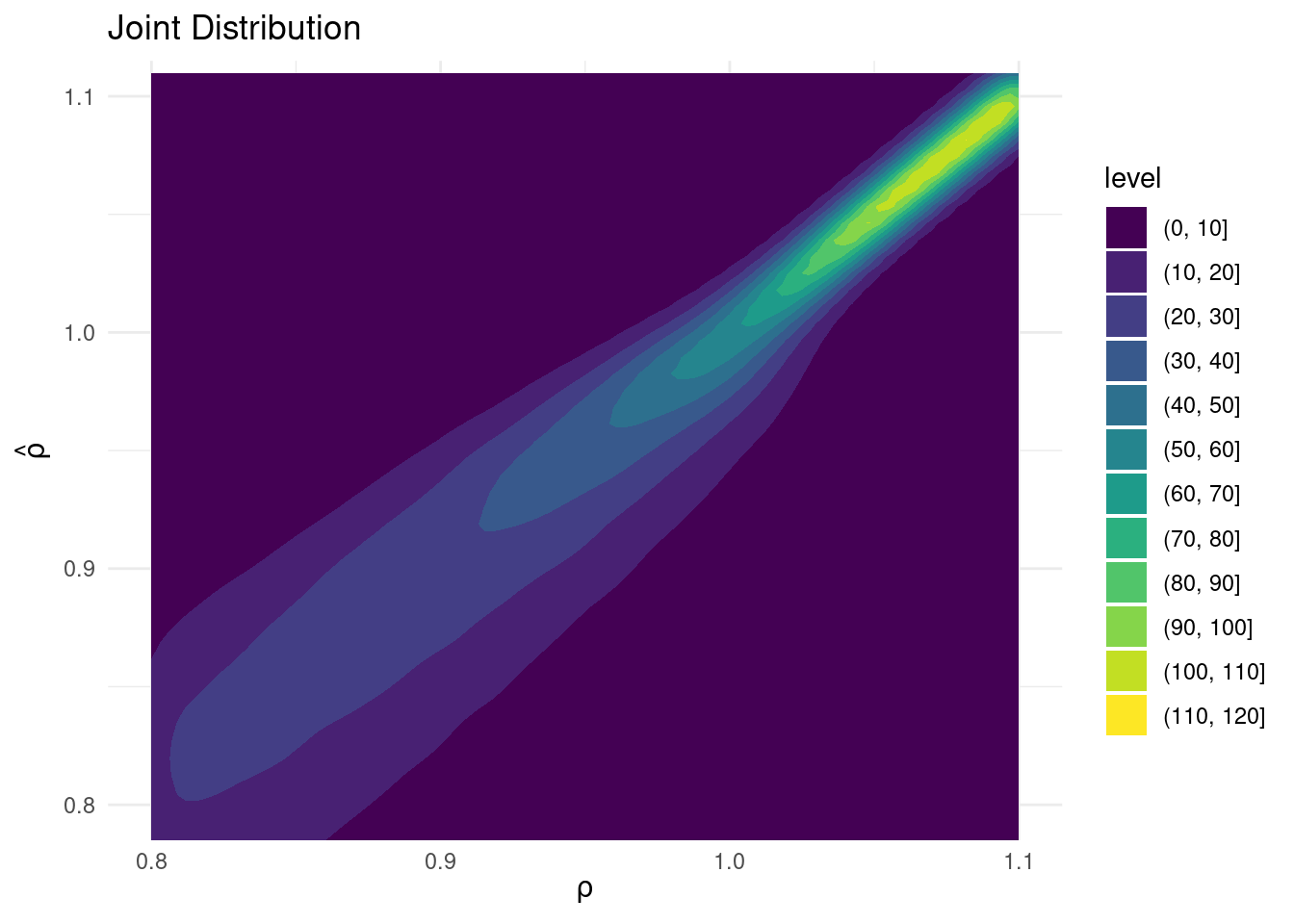
joint |>
  filter(rho_hat >= 0.995 & rho_hat < 1.005) |>
  ggplot(aes(x = rho)) +
  geom_histogram(binwidth = 0.01, fill = "skyblue", color = "black") +
  labs(title = expression(hat(rho) == 1),
       x = expression(rho),
       y = "Frequency") +
  theme_minimal()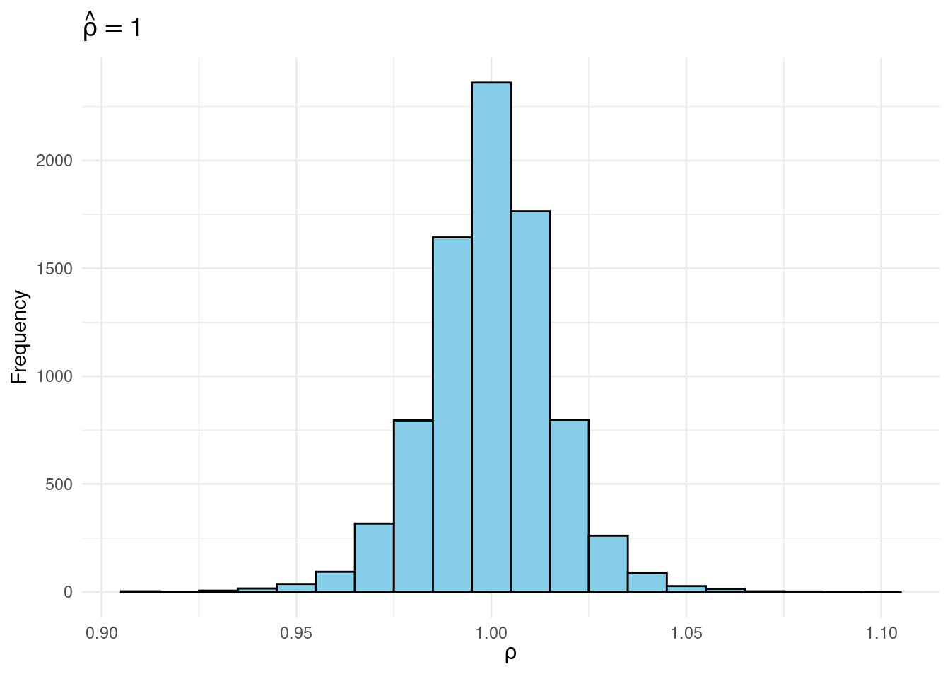
joint |>
  filter(rho == 1) |>
  ggplot(aes(x = rho_hat)) +
  geom_histogram(binwidth = 0.01, fill = "skyblue", color = "black") +
  labs(title = expression(rho == 1),
       x = expression(hat(rho)),
       y = "Frequency") +
  theme_minimal()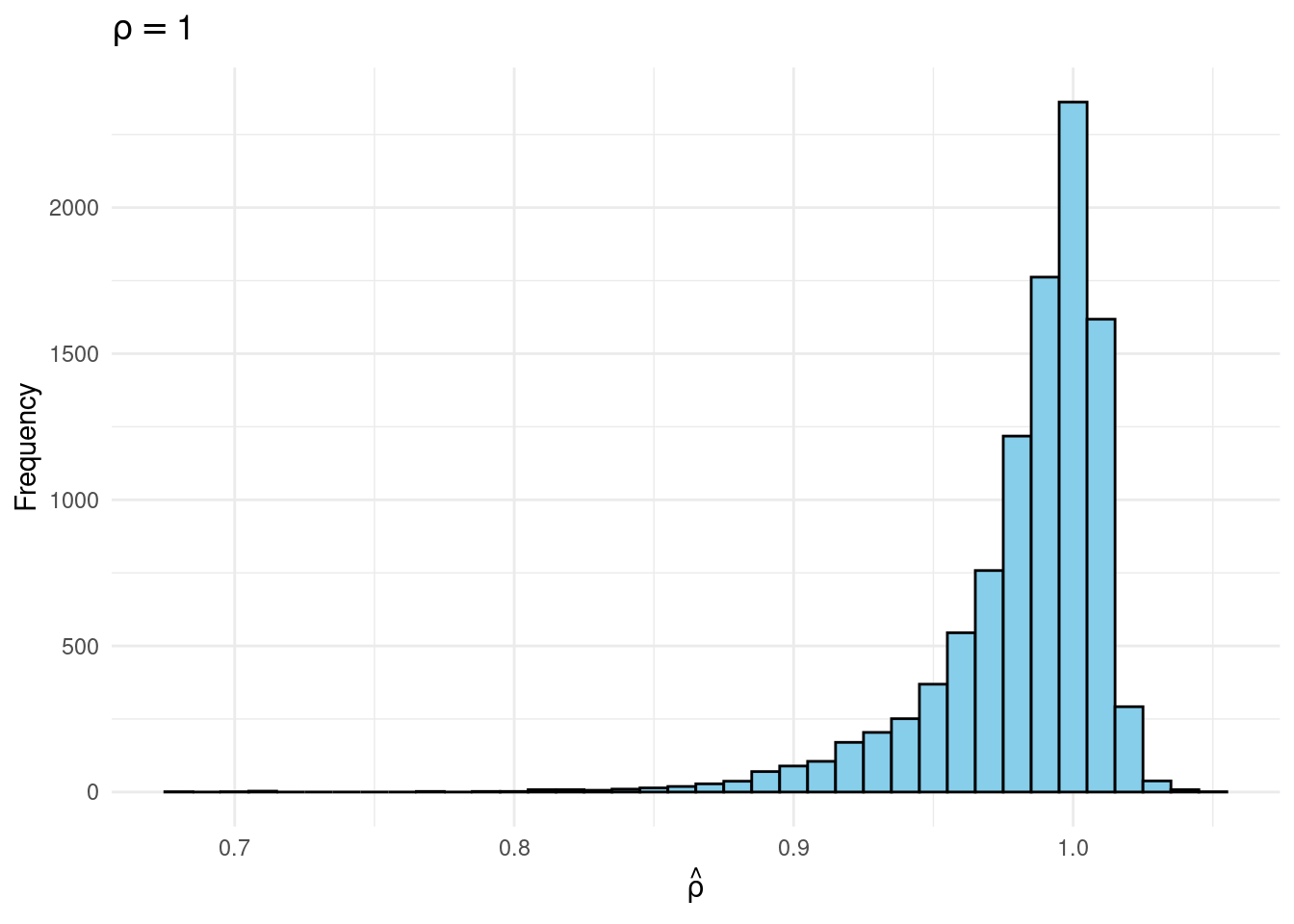
# Function that makes the preceding two plots, puts them side-by-side and lets
# the user specify the value of rho/rho_hat that we condition on:
plot_Bayes_vs_Freq <- \(r) {
  p1 <- joint |>
    filter(rho_hat >= r - 0.005 & rho_hat < r + 0.005) |>
    ggplot(aes(x = rho)) +
    geom_histogram(aes(y = after_stat(density)),
                   binwidth = 0.01, fill = "skyblue", color = "black") +
    geom_vline(xintercept = r, color = "red", linetype = "dashed", linewidth = 1) +
    labs(title = bquote(hat(rho) == .(round(r, 3))),
         x = expression(rho)) +
    theme_minimal()

  p2 <- joint |>
    filter(rho >= r - 0.005 & rho < r + 0.005) |>
    ggplot(aes(x = rho_hat)) +
    geom_histogram(aes(y = after_stat(density)),
                   binwidth = 0.01, fill = "skyblue", color = "black") +
    geom_vline(xintercept = r, color = "red", linetype = "dashed", linewidth = 1) +
    labs(title = bquote(rho == .(round(r, 3))),
         x = expression(hat(rho))) +
    theme_minimal()

  p1 + p2
}

plot_Bayes_vs_Freq(0.98)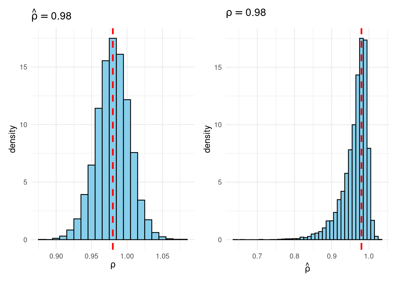
plot_Bayes_vs_Freq(0.99)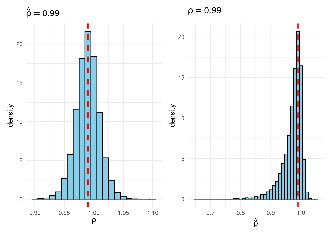
plot_Bayes_vs_Freq(1.0)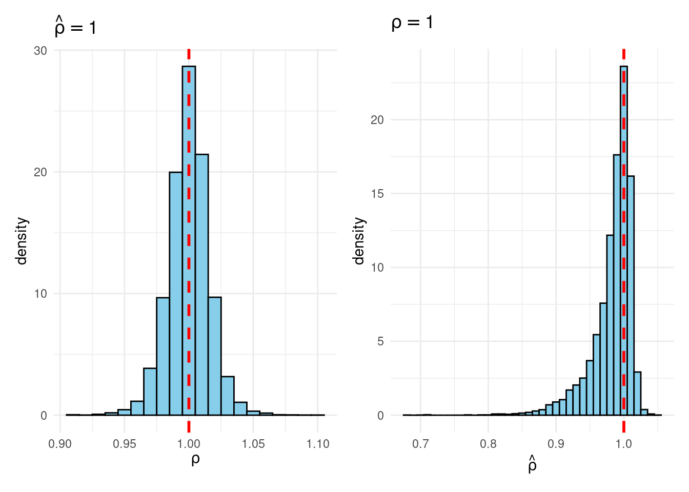
plot_Bayes_vs_Freq(1.01)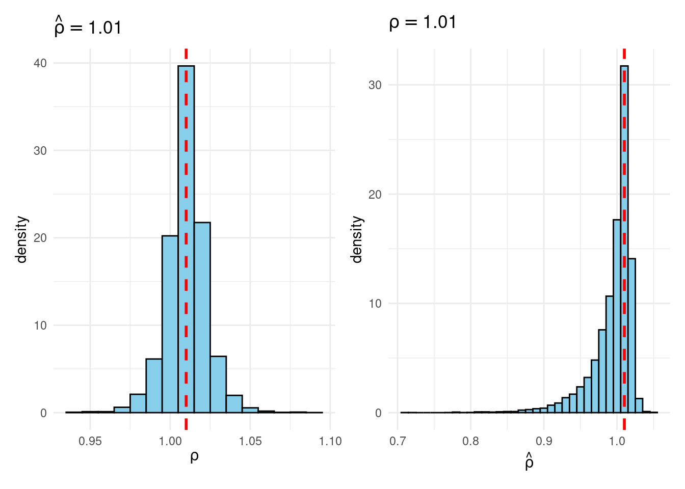
plot_Bayes_vs_Freq(1.02)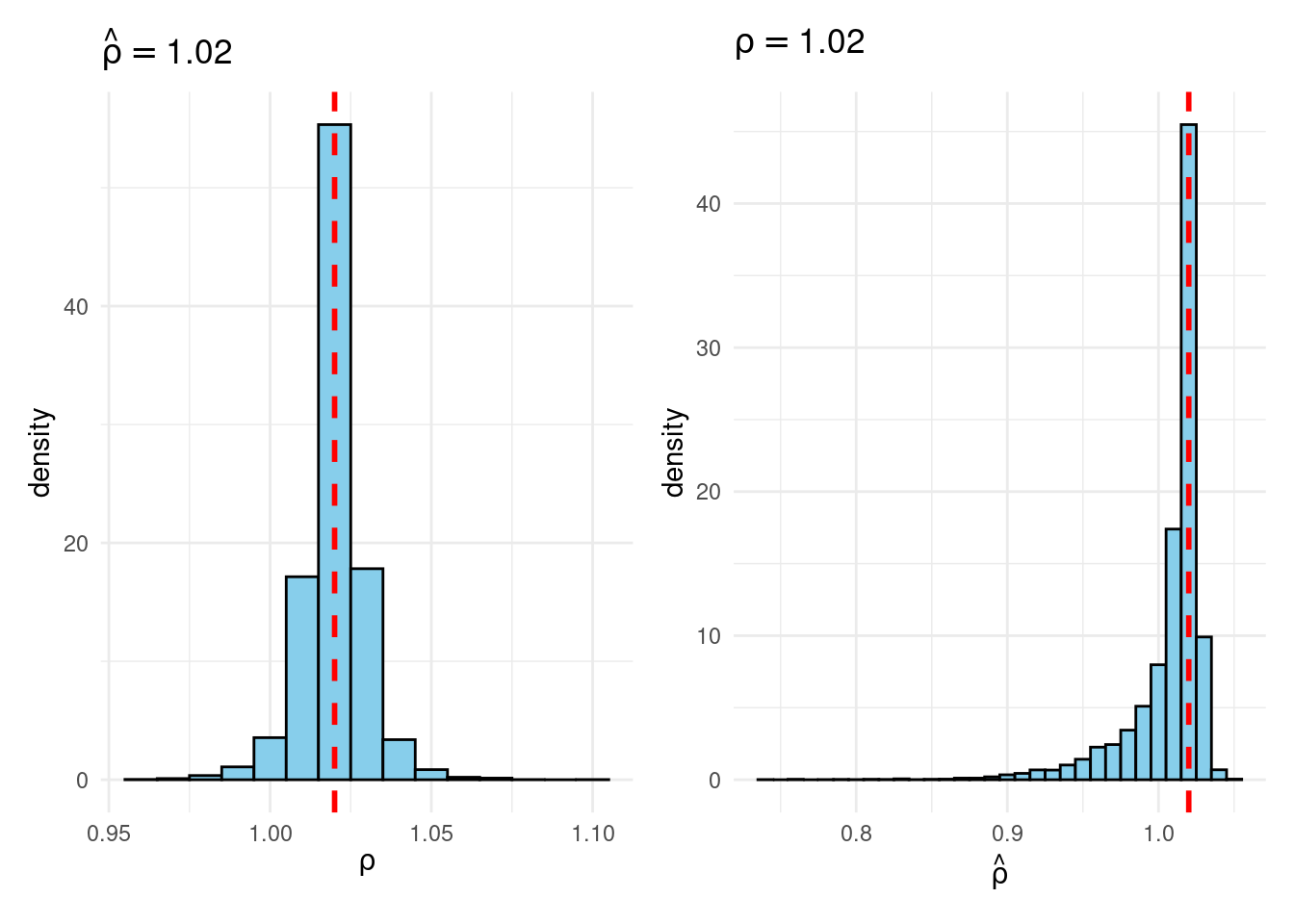
A detailed discussion of the likelihood principle would require at least a whole post of its own. If you want to learn more, I highly recommend the classic monograph by Berger & Wolpert.↩︎
For further discussion of Sims and Uhlig’s illuminating simulation experiment, see Chapter 6 of Poirier.↩︎